Classifying bugfix commits with ML.NET

This article is a case study in using ML.NET to train and select an optimal binary classification model for use in classifying code commits as bugfix or non-bugfix related based on their commit metadata.

This is a modified version of my master’s project’s final summary report and so the tone, style, and approach will be slightly different than my other writing. Where possible I will link to other articles of mine detailing concepts in more detail. Nonetheless, I believe you should find it an interesting illustration of why I find ML.NET to be an effective machine learning library and some creative uses of Phi-3 LLMs to help draft a pre-review training dataset.

This content is also available as a YouTube video

Project Objective and Context

Software engineers, data scientists, data engineers, and other technology professionals use source control management systems such as git to track changes to repositories of code over time. These changes are called commits and relate to one or more files and include one or more file and line of code that is modified. Often there will be many additions and deletions across several files. Each of these commits contains information about when it occurred, who performed it, and the message they used to describe the overall set of changes.

To help analyze the history of git-based codebases I’ve been developing a tool called GitStractor. This project can extract data from any git repository regardless of programming languages used and store that data in a set of CSV files. These CSV files can then be ingested by an analytics notebook or data visualization tool to visualize the structure of the project and how it had changed over time.

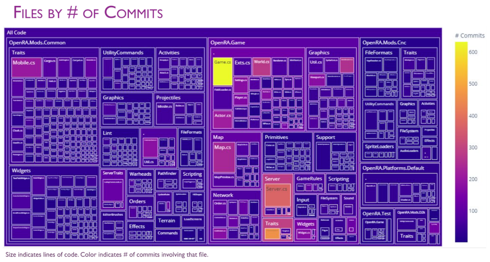
GitStractor has proved effective in its ability to glean and communicate insight from code, but it was not able to adequately communicate important information on software quality without a way of determining whether a commit was bugfix-related or non-bugfix related.

This project exists to train such a binary classification model in such a way that maximizes the resulting model’s F1 Score while retaining high precision for bugfix predictions in order to minimize the odds of false positives erroneously flagging good areas of code as problematic. Such mistakes could compromise the reputations of individuals or teams.

Because GitStractor is .NET-based (after an initial Python implementation proved too slow), the ideal model should run under ML.NET either as a ML.NET native model or as a model importable into ML.NET using Open Neural Network eXchange (ONNX) format.

Data Preparation

In order to train a supervised model to classify commits as bugfix or non-bugfix I needed a suitable labelled dataset with information on individual commits along with their classification as a bugfix or non-bugfix. Unfortunately, no suitable dataset existed so I needed to create one.

Base Dataset

A small initial dataset of commits from open source and smaller side project repositories was selected as the source of commits for the initial training set. These commits came from the following repositories:

• ML.NET – Microsoft’s machine learning library for .NET applications
• Polyglot Notebooks / .NET Interactive – A collection of kernels integrated into Jupyter Notebooks allowing for additional languages such as C#, F#, PowerShell, and SQL.
• GitStractor – The tool used to extract git information to CSV files (because of course I analyzed the tool with itself).
• Emergence – A science fiction roguelike game development project I was working on at one time.
• Wherewolf – A probabilistic model of the One Night Ultimate Werewolf card game I’m currently developing as time allows.

Each of these repositories is a repository that is under the MIT License and is an example of public code I have personal familiarity with. This personal familiarity was important because of how the training labels were generated as we’ll discuss shortly.

Each commit included details on its unique hash (Sha), the author and committer of the commit (committer may sometimes be different than the author and represents the person who committed changes by another author), the commit message, a count of work items mentioned, a count of added, deleted, and modified files and lines of code, and a boolean indicating if the commit represents a merge commit merging commits from one branch into another.

Generating Preliminary Labels

A label column was added to the dataset indicating whether or not the commit represented a bugfix commit. The initial value of this column came from using LLamaSharp to interact with a Phi-3 Mini 4k Instruct large language model (LLM) running on-device on a Linux machine using an RTX 4070 graphics card and CUDA 12.

The prompt given to the LLM instructed it to produce a JSON output including the prediction and a reason for that prediction. This response was then deserialized into an object and the PredictedLabel and Reason columns were added to the dataset.

With optimal settings, this interaction took 0.7 seconds per commit, which was still unacceptably long for production usage where thousands of commits may be present.

EDA and Data Sampling

Once all 5 repositories had their data extracted and preliminary labels generated, a notebook was used to load the separate 5 data files, merge each one together with the predicted labels (stored in a separate CSV to prevent overwriting the source file), and then merge all 5 resulting DataFrame objects together into a single unified DataFrame.

From there, rows containing NA values were dropped, and exploratory data analysis was used to detect outliers and correlations.

There were extreme outliers in terms of files and lines added / removed. However, I chose not to address these at the data preparation stage because extreme values exist in real-world repositories and the problem would be better solved by using a normalizing transform such as a min / max or standard scalar as part of the model training pipeline.

Some feature engineering occurred during this process with new columns being added for time of day, day of week, and month of year binning. However, EDA revealed that activities on repositories occurred across multiple timezones and we could not accurately normalize commit times without knowing the local time zone for the committer. As a result, all time and date related values were dropped to ensure the model would not be biased by time zone differences.

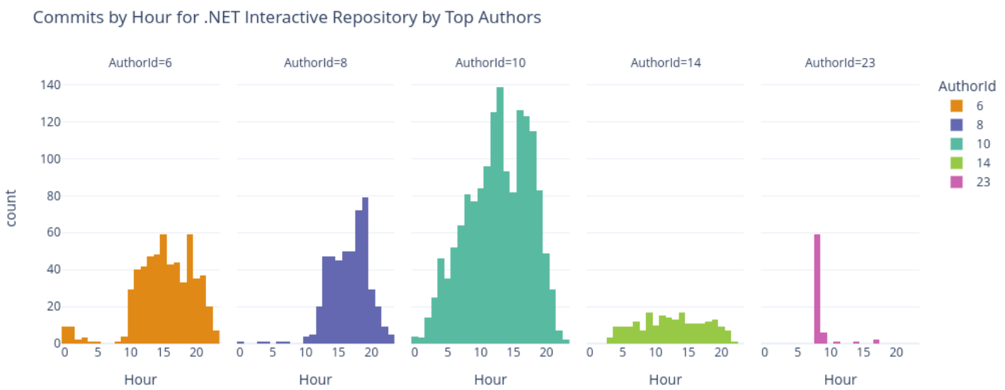
All information about the author and committer was dropped as well because these fields may be relevant for models trained for a specific repository, they would not be relevant for a generalized predictive model and may exhibit unfair biases against individuals.

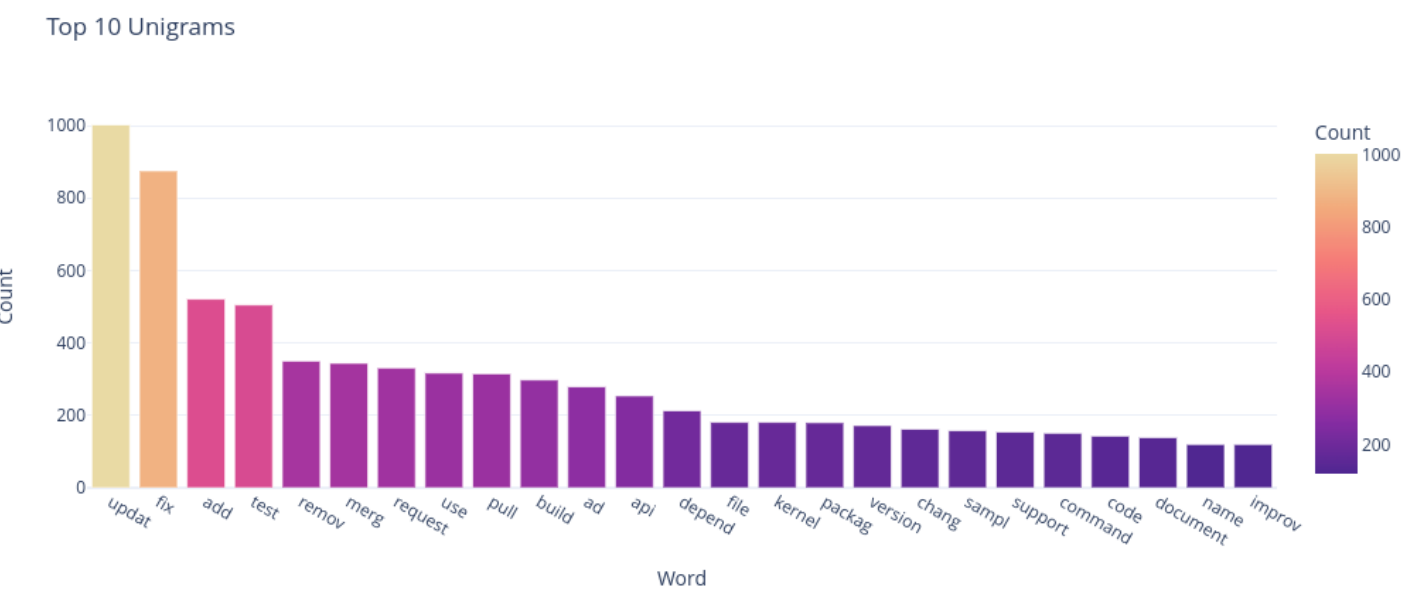
Correlation analysis revealed some correlations with the IsBugFix column (our label column), but no truly strong correlations existed that seemed likely to drive a suitable model. Extracting unigrams and bigrams from the message helped with this and showed that natural language processing would be critical to a well-performing model.

Since the initial training labels were generated by an LLM, they were not suitable for usage in model training without human review and correction. The overall dataset consisted of 6576 commits which would be too prohibitive for manual review given the scope of this project.

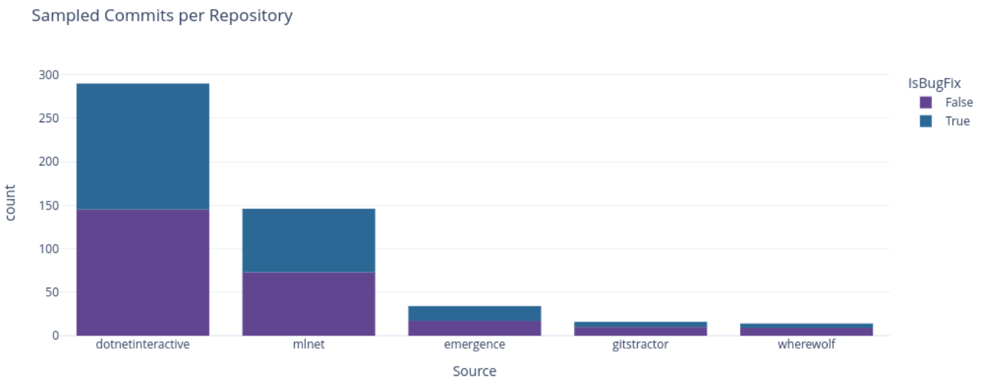
To address this, I sampled down to 500 commits by using a representative stratified sampling strategy where each repository included in the experiment had a relative portion of its commits selected for the final training data selection. This selection was further stratified to ensure that each repository had an equal count of bugfix and non-bugfix commits from the initial predictions as shown here:

The 500 rows in the final dataset were then manually reviewed by myself (note that I have familiarity with all 5 repositories and 20 years of experience as a software engineer to qualify me to do this) and corrected values were saved in the Label column. Having an initial PredictedLabel column and a corrected Label column allowed for evaluating the initial classifier’s accuracy metrics for comparison purposes.

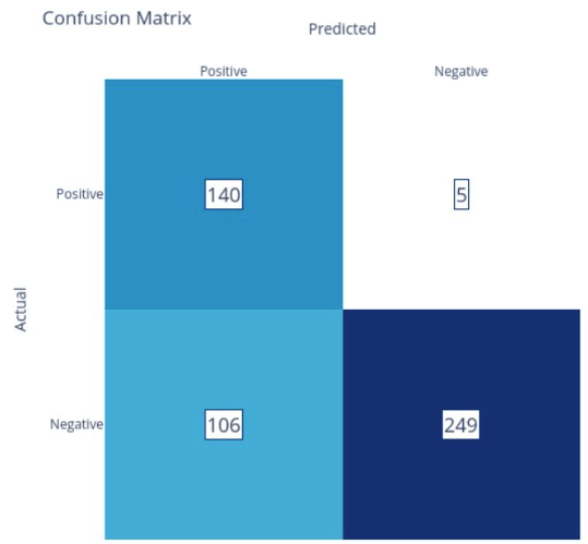
With the final labels in place, additional exploratory data analysis was performed on the final sample. The resulting sample did have a class imbalance with 71% of the rows indicating non-bugfix commits while 29% did involve bugfixes. This class imbalance occurred because the Phi-3 LLM’s positive precision was low, leading to a high number of false positives in the stratified sample. However, the results were within tolerances to move on, with a caveat that additional training data may be needed to generate the best results.

In all other respects, the final model’s distributions resembled that of the original dataset before sampling, so all unnecessary columns were dropped and a final training file was created for model training.

Model Training & Evaluation

The model training process was primarily conducted in a single Polyglot Notebook (.NET kernels added on to Jupyter Notebooks) using ML.NET.

These technologies are high quality, but lacked critical components such as a graphical confusion matrix and other charting capabilities. To address this, I created 4 small machine learning libraries for this project under the operating label of MattEland.ML, MattEland.ML.Interactive, MattEland.ML.Charting, and MattEland.ML.DataFrame. These libraries are not yet ready for public usage, but may see refinement and either become a full open-source project or I may seek to find a way of getting them incorporated into the main ML.NET project.

Yes, I really am nerdy enough that I prototyped open-source libraries to support this project.

Initial ML.NET AutoML Models

One ML.NET’s advantages is a powerful AutoML library that evaluates many different model trainers, model pipelines, and model hyperparameters, so I decided to start my modelling process with that.

Initial models exhibited F1 Scores 0.65 or higher with positive precisions over 70%.

Note: all metrics in this section are representative of verification metrics. Models were trained using 5 fold cross validation on 80% of the data with the remaining 20% of the data being used as final verification data on the model selected by AutoML using cross validation against 80% of the training data.

As expected, the early models were primarily fast trees and fast forests, ML.NET’s implementation of decision trees and random forests respectively.

These early AutoML models also generated training pipelines involving missing value imputers, converting boolean values to floating point values for ML.NET consistency, text transformation / n-gram extraction, and concatenating all feature columns together for ML.NET processing.

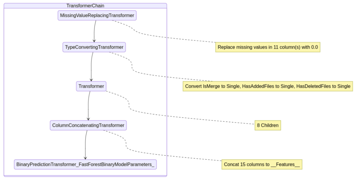
However, these text processing pipelines did not clean sensitive values from the message column or remove stop words. To address this, the project moved from simple AutoML to AutoML with manual control over the pipeline. I then implemented my own processing pipeline that added in a custom TextNormalizingTransformer step.

This pipeline replaced all numbers and URLs in the Message column with sentinel values. This reduced metrics slightly, but prevented models from overfitting on word or character n-grams present in URLs or issue numbers.

From there, the pipeline was repeated a number of times focused on each of the common ML.NET binary classification models supported by AutoML: fast forest (random forest), fast tree (decision tree), LGBM gradient boosted, L-BFGS logistic regression, and SDCA logistic regression. Each model trainer was given 10 sample iterations for hyperparameter tuning for later comparison against each other and other models from other platforms

Other Models Considered

In addition to the basic ML.NET models, other models were evaluated for comparison.

As of ML.NET 2.0, ML.NET supports text classification by fine-tuning BERT models. A Roberta model was fine-tuned on the training data, but this model had a low F1 score of 0.37 due to a positive recall of only 0.25.

Six model trainers using Python and SciKit-Learn were also evaluated using random forest, support vector classifier, logistic regression multinomial NB, KNN, and a MLP neural network algorithms. These models did not have as extensive hyperparameter tuning or pipeline development as my ML.NET alternatives, but the experiment in Python was used to flag potential models that were not considered using ML.NET (ML.NET and SciKit-Learn models are generally comparable in their output model quality since the underlying math is identical). If a high accuracy model was discovered that supported ONNX export it might be considered for the final model. Unfortunately, none was discovered.

The initial Phi-3 LLM should also be listed here for consideration. While the model had an F1 Score of 0.71, it’s positive precision was only 56%.

Finally, Azure Machine Learning Studio’s AutomatedML API was used to train a pair of models – one using standard binary classification and the other with deep learning enabled. Both models used ensemble methods involving random forests and XGBoost models, but had F1 scores around 0.58, making them less viable than the ML.NET models.

Final Model Hyperparameter Tuning

Given the observations from various early experiments, a series of final models were trained using ML.NET for with targeted hyperparameter tuning around a specific targeted range of values using an ECI Cost Frugal tuner algorithm built for hierarchical hyperparameter tuning exploration with a goal of minimizing compute requirements. These training efforts also dedicated additional compute time to the tuning experiment to optimize the selected model.

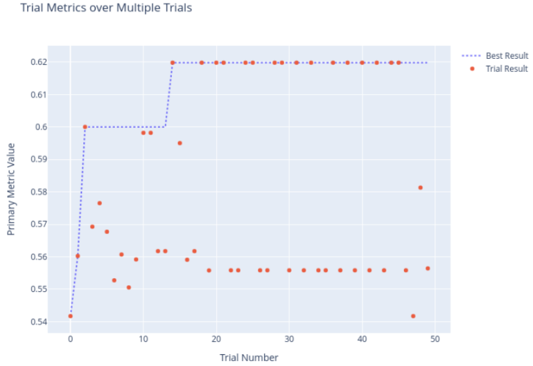
This experimentation was done using a fast forest, a light gradient boosted model, simple logistic regression, a field-aware factorization machine, Microsoft’s local deep learning SVM, an averaged perceptron, and a linear SVM. The final model metrics are listed here:

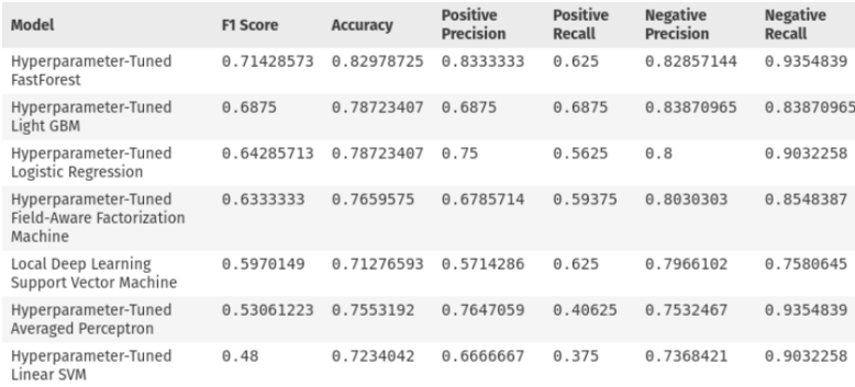
Final model selection was close between the fast forest, light GBM, and logistic regression models. In this decision models were evaluated by their F1 score, positive precision, and evaluations of their permutation feature importances and hyperparameter settings.

The random forest used 3 trees with up to 10 leafs each, and restricted its training to using 72% of the features for tree forming. Its most relevant PFI factors all appeared to be character bigrams or trigrams related to substrings found in words like “Fix” or “Issue”. The model did not seem to value characteristics of the non-message columns.

The light GBM model had similar settings to the random forest, using a learning rate of 0.5. Like the random forest it looked primarily for character strings, but the strings made less sense. Additionally, this model took significantly longer to train and likely wouldn’t scale well during training with additional data.

The logistic regression model had an L1 regularization value of 0.08 and a L2 regularization of 0.0003. This model valued the word count, looked for words like fix, bad, and update, and looked to see if the change included any new files. While its performance was slightly worse than the random forest, this model may be more likely to generalize well on data from repositories outside of the 5 used for training. However, its positive precision is 8% worse and F1 score is 0.7 lower as well.

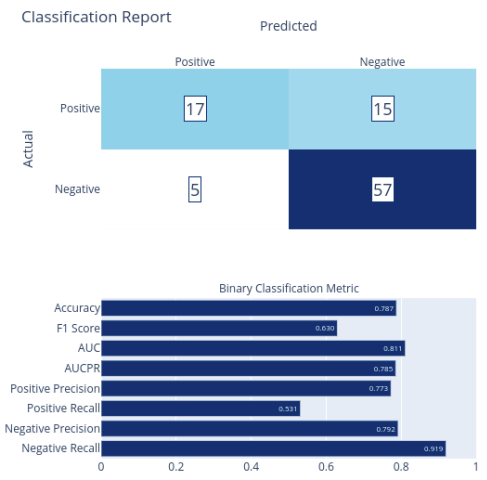
Thankfully, logistic regression in ML.NET is a calibrated model whereas random forests are non-calibrated. This means that logistic regression provides both a predicted label and a probability with 1 being certain to be a bugfix and 0 being certain to be non-bugfix.

Not only is the probability an additional data point for potential inclusion in GitStractor visuals, but it enables me to arbitrarily set a threshold on predictions in order to further improve model precision. Although I’ve not yet implemented a precision-recall curve chart for ML.NET, you would be following that same precision-recall curve by increasing the threshold for positive classification. This would then improve the model’s positive precision while decreasing the model’s positive recall.

Model Deployment

The three best models identified during training were saved to .zip files (ML.NET’s file format of choice) and the logistic regression model was then embedded into GitStractor.

I then implemented a new git commit observer that transformed the raw commit information into the input format the model expected and defined my output object consisting of the predicted label and probability.

This allows GitStractor to classify incoming commits in real-time and serialize the predicted label and its probability to the generated CSV file for later analysis.

Because logistic regression is relatively fast and simple, I have confidence that I have not overfit my training data. Additionally, its performance allows me to classify entire repositories of git commits in the time the Phi-3 mini instruct 4k LLM took to classify several commits previously. Furthermore, I have reason to believe I could parallelize this extraction process if I needed to because ML.NET allows me to use a performant thread-safe PredictionEnginePool class.

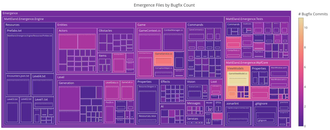
While I am still early on in my analysis of the outputted data and calibration of the best prediction cutoff to use for this model, I am already starting to see value for the model in identifying areas of code in need of remediation or additional testing.

Conclusion

I view this project as a success in regards to exploring the depths of machine learning, developing workflows around training ML.NET models in Polyglot Notebooks, and training an effective binary classifier for commit bugfix predictions.

I hope to expand on this GitStractor tool in the future, but if there’s any particular aspect of this project you find intriguing, please let me know and I’ll provide additional details.

Finally, on a personal note, I’m quite proud that the .NET technologies I love were part of my research efforts and the master’s of science in data analytics degree I now hold.